Motion by Mean Curvature

This post explains and implements the MBO (Merriman-Bence-Osher) scheme for diffusion generated motion by mean curvature [1]. The MBO scheme is a strikingly simple method to model mean curvature flow, also known as motion by mean curvature. I first provide a brief introduction to the phenomenon of motion by mean curvature and the physical contexts in which it arises. I then explain and motivate one possible implementation of the MBO scheme and use this implementation to produce some cool pictures and videos.

Introduction

To illustrate motion by mean curvature, suppose that \(\Omega \subset \mathbb R^2\) is a subset of the plane partitioned into two parts separated by a boundary \(\partial\), as in the following picture.

Figure 1: A rectangular region \(\Omega \subset \mathbb R^2\) partitioned into two parts (black and white) separated by a boundary \(\partial\).

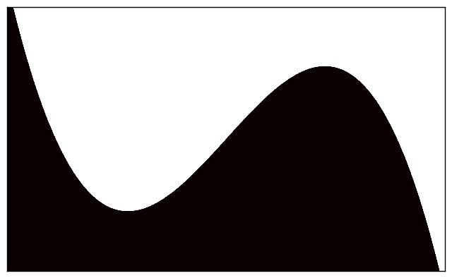
A rigorous discussion of mean curvature is beyond the scope of this post. It suffices to note that the mean curvature of a surface embedded in a higher dimensional space is a local measure of how “curvy” the surface is at any particular point. In the present context, our “surface” is just the one-dimensional curve \(\partial\), the ambient space is \(\mathbb R^2\), and mean curvature reduces to the same notion of curvature that one encounters in an introductory vector calculus class. The boundary \(\partial\) is said to “move by mean curvature” or “evolve under mean curvature flow” if a point \(\mathbf r\) on \(\partial\) moves in a normal direction to \(\partial\) with velocity proportional to the mean curvature (i.e., curvature) of \(\partial\) at \(\mathbf r\). In other words, points at which the boundary is “curvy” will move faster than points at which the boundary is relatively straight. For example, consider the following images.

Figure 2: The evolution of \(\Omega\) as the boundary \(\partial\) moves by mean curvature.

(a) \(\Omega\) at an initial time.

(b) \(\Omega\) after the boundary \(\partial\) has evolved under mean curvature flow for some time.

(c) The initial and final configurations of \(\Omega\) superimposed.

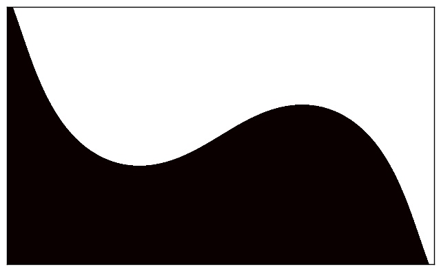
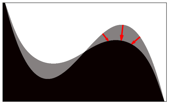
Figure 2a shows \(\Omega\) at an initial time and Figure 2b shows \(\Omega\) after the boundary \(\partial\) has evolved under mean curvature. In Figure 2c, the initial and final configurations of \(\Omega\) are superimposed, and red arrows indicate the motion of a few select points along the boundary. Notice that points at which \(\partial\) has high curvature travel faster and cover greater distance than points at which \(\partial\) has relatively low curvature.

The phenomenon of motion by mean curvature is observed in several physical applications. For example, certain distinct fluids do not intermix but are instead separated by a thin region known as a “diffuse interface” that evolves under mean curvature flow. A second example occurs in the context of metallurgy, where a metal undergoing phase transition develops an interface between distinct phases (e.g., liquid and solid) that obeys motion by mean curvature. An understanding of mean curvature flow is thus necessary for modeling certain physical phenomena. Motion by mean curvature is of personal interest for an additional reason. The technique I employ to model mean curvature flow, the MBO (Merriman-Bence-Osher) scheme for diffusion generated motion, was subsequently adapted into a semi-supervised learning algorithm [2] that was the subject of my undergraduate senior thesis. I undertook the current project to better understand the MBO scheme in its original context of mean curvature flow and to generate some cool pictures for my thesis.

MBO Scheme for Diffusion Generated Motion by Mean Curvature

The MBO scheme for diffusion generated motion is a remarkably simple technique to model mean curvature flow. Suppose that \(\Omega\) is a subset of the plane partitioned into two parts as previously explained. Let the “characteristic function” \(\chi : \Omega \times T \rightarrow \mathbb R\), where \(\chi(\mathbf r, t) = 0\) if \(\mathbf r\) belongs to the first part in the partition at time \(t\), and 0 if it belongs to the second part (we sometimes omit the argument \(t\) for convenience). The MBO scheme first diffuses the characteristic function \(\chi\) for some short time step, then thresholds by rounding \(\chi(\mathbf r)\) to 0 or 1 for all points \(\mathbf r \in \Omega\). By alternating between diffusion and thresholding steps, the MBO scheme approximates the motion by mean curvature of the boundary \(\partial\) [3] [4]. An outline of the scheme is provided below.

Input: characteristic function \(\chi\), time step \(k\)

1. until convergence:
   1. Diffuse \(\chi\) for \(k\) units of time.
   2. \(\forall \mathbf r \in \Omega, \chi(\mathbf r) \gets \begin{cases} 1 & \mbox{if } \chi(\mathbf r) \geq \frac 12,\\ 0 & \mbox{otherwise.}\end{cases}\)
2. return \(\chi\)

Output: updated \(\chi\)

For simplicity, I have outlined and implemented the MBO scheme for a two-dimensional domain partitioned into two parts. However, the scheme is quite flexible and may be generalized in a straightforward manner to higher dimensional domains partitioned into an arbitrary number of parts.

Diffusion

The most expensive aspect of the MBO scheme, in terms of both computational cost and implementation effort, is the diffusion of the characteristic function \(\chi\). I will briefly introduce the diffusion equation and will describe one simple numerical method to solve it.

Diffusion Equation

Suppose that \(\Omega \subset \mathbb R^2\) is a bounded and simply connected spatial region occupied by a diffusing material. Let \(T = [0, \infty)\) denote some range of time and let \(\rho : \Omega \times T \rightarrow \mathbb R\), where \(\rho(\mathbf r, t)\) denotes the concentration of the diffusing material at position \(\mathbf r \in \Omega\) and time \(t \in T\). The physics of diffusion is governed by the diffusion equation

\[ \frac{\partial \rho}{\partial t} = D \Delta \rho, \]

where the “diffusion coefficient” \(D\) has dimensions \(\left[\frac{(length)^2}{time}\right]\) and determines the rate of diffusion of the material in question (we shall assume for the sake of simplicity that \(D\) is constant, although it may in general be a function of the concentration \(\rho\) and position \(\mathbf r\)). The diffusion of heat obeys the same law as a diffusing material. Thus, the above equation is referred to as the “heat equation” when \(\rho\) denotes temperature rather than concentration.

In addition, we’ll assume we have complete knowledge of \(\rho\) on \(\partial\) given by the Dirichlet boundary conditions

\[ \rho(\mathbf r) = f(\mathbf r) \]

for \(\mathbf r \in \partial\) (where \(f : \partial \rightarrow \mathbb R\) is known). This assumption guarantees a unique solution to the diffusion equation above.

Numerical Scheme

TL;DR: \eqref{eq:expanded_poisson_system} is equivalent to \eqref{eq:poisson_system}. Skip to the implementation.

This section presents one possible method for numerically solving the diffusion equation using a finite difference scheme and the Method of Lines. For simplicity, assume that \(\Omega = [a, b] \times [c, d]\) is a rectangular subset of the plane and divide the intervals \([a, b]\) and \([c, d]\) into \(m + 1\) and \(n + 1\) subintervals of length \(h_x = (b - a) / (m + 1)\) and \(h_y = (d - c) / (n + 1)\), respectively. Then define \(x_i := a + ih_x\) for \(i=0, 1, 2, \ldots, m+1\) and \(y_j := c + j h_y\) for \(j = 0, 1, 2, \ldots, n+1\). At each meshpoint \((x_i, y_j)\), we can approximate \(\Delta \chi\) using the second-order central finite difference

\[ \Delta \chi(x_i, y_j) = \chi_{xx}(x_i, y_j) + \chi_{yy}(x_i, y_j) \approx \frac{\chi_{i,j+1} - 2\chi_{i,j} + \chi_{i,j-1}}{h_x^2} + \frac{\chi_{i+1,j} - 2 \chi_{i,j} + \chi_{i - 1, j} }{h_y^2}, \]

where \(\chi_{i,j} := \chi(x_i, y_j)\) for \(0 \leq i \leq n+1, 0 \leq j \leq m+1\). Setting the diffusion coefficient \(D = 1\), we have

\begin{equation} \label{eq:expanded_poisson_system} -\frac{\partial \chi}{\partial t} (x_i, y_j) \approx -\frac{1}{h_y^2}\chi_{i-1,j} - \frac{1}{h_x^2} \chi_{i, j-1} + \left(\frac{2}{h_x^2} + \frac{2}{h_y^2}\right) \chi_{i,j} - \frac{1}{h_x^2} \chi_{i,j+1} - \frac{1}{h_y^2} \chi_{i+1,j} \end{equation}

for \(1 \leq i \leq n, 1 \leq j \leq m\). The above system of equations may be conveniently expressed in matrix notation by defining

• the reshaped characteristic function \(\vec\chi(t) \in \mathbb R^{nm}\), \[ \vec\chi(t) := \left(\chi_{1,1}(t), \chi_{2,1}(t), \ldots, \chi_{n,1}(t), \chi_{1,2}(t), \chi_{2,2}(t), \ldots, \chi_{n,2}(t), \ldots, \chi_{1,m}(t), \chi_{2,m}(t), \ldots, \chi_{n,m}(t)\right)^T, \]

• the tridiagonal matrix \(B_{h_x, h_y} \in \mathbb R^{n \times n}\), \[ B_{h_x, h_y} := \begin{pmatrix} \frac{2}{h_x^2} + \frac{2}{h_y^2} & -\frac{1}{h_x^2} & & & & \\
  -\frac{1}{h_x^2} & \frac{2}{h_x^2} + \frac{2}{h_y^2} & \ddots & & & \\
  & \ddots & \ddots & -\frac{1}{h_x^2} & & \\
  & & -\frac{1}{h_x^2} & \frac{2}{h_x^2} + \frac{2}{h_y^2} & -\frac{1}{h_x^2} & \\
  & & & -\frac{1}{h_x^2} & \frac{2}{h_x^2} + \frac{2}{h_y^2} \\
  \end{pmatrix}, \]

• the block-tridiagonal matrix \(A_{h_x, h_y} \in \mathbb R^{mn \times mn}\), \[ A_{h_x, h_y} := \begin{pmatrix} B_{h_x, h_y} & -\frac{1}{h_y^2}I_n & & & & \\
  -\frac{1}{h_y^2}I_n & B_{h_x, h_y} & \ddots & & & \\
  & \ddots & \ddots & -\frac{1}{h_y^2}I_n & & \\
  & & -\frac{1}{h_y^2}I_n & B_{h_x, h_y} & -\frac{1}{h_y^2}I_n & \\
  & & & -\frac{1}{h_y^2}I_n & B_{h_x, h_y} \\
  \end{pmatrix}, \]

• and boundary conditions \(\mathbf b \in \mathbb R^{nm}\), \[ \mathbf b := \frac{1}{h_y^2} \begin{pmatrix} \chi_{1,0} \\\ \chi_{2,0} \\\ \vdots \\\ \chi_{n,0} \\\ 0 \\\ \vdots \\\ 0 \\\ \chi_{1,m+1} \\\ \chi_{2,m+1}\\\ \vdots \\\ \chi_{n,m+1} \end{pmatrix} \; + \; \frac{1}{h_x^2} \begin{pmatrix} \chi_{0,1} \\\ 0 \\\ \vdots \\\ 0 \\\ \chi_{n+1,1} \\\ \chi_{0,2} \\\ 0 \\\ \vdots \\\ 0 \\\ \chi_{n+1,2} \\\ \vdots \\\ \chi_{0,m} \\\ 0 \\\ \vdots \\\ 0 \\\ \chi_{n+1,m} \end{pmatrix}. \]

You can verify that the (i + (j-1)n)^th coordinate of \(A_{h_x,h_y}\vec\chi - \mathbf b\) is just the right-hand side of \eqref{eq:expanded_poisson_system}. To approximate the left-hand side, let \(t_0\) denote the initial time and \(t_1 = t_0 + k\) denote the final time after time step \(k\) has elapsed. Using implicit Euler method, we approximate

\[ \frac{\vec\chi(t_0) - \vec\chi(t_1)}{k} \approx A_{h_x,h_y}\vec\chi(t_1) - \mathbf b. \]

Rearranging terms, we have the linear system

\begin{equation} \label{eq:poisson_system} \vec \chi(t_0) + k\mathbf b \approx \left(I_{nm} + kA_{h_x, h_y}\right) \vec\chi(t_1), \end{equation}

which we solve for the diffused characteristic function \(\vec\chi(t_1)\).

Implementation

All matrices are sparse. The matrix \(A_{h_x, h_y}\) may be conveniently constructed as

\[ I_m \otimes B_{h_x, h_y} - \frac{1}{h_y^2} (C \otimes I_n), \]

where \(C \in \mathbb R^{m \times m}\) has ones on the super- and sub-diagonals and zeroes elsewhere, and \(\otimes\) denotes the Kronecker product. The matrix \(\left(I_{nm} + kA_{h_x, h_y}\right)\) is symmetric positive-definite. We use Conjugate Gradient Method, a solver for symmetric positive-definite linear systems that is significantly faster than scipy’s generic sparse solver. The diffusion equation is an example of Poisson’s equation, an elliptic partial differential equation. While more efficient methods for solving Poisson’s equation exist, CG Method enjoys the merits of simplicity and ease of implementation and is fast enough for the current application.

Now let’s start coding. We first define the characteristic function \(\chi\) for \(\Omega\) at an initial time \(t_0\). I use a cubic polymomial to serve as the boundary \(\partial\) in \(\Omega\) because it is both visually appealing and has non-constant curvature. I also write a convenient function for plotting \(\chi\).

import numpy as np
import scipy.sparse as sp
import scipy.sparse.linalg as splin
import matplotlib.pyplot as plt
from mpl_toolkits.axes_grid1 import make_axes_locatable
import math

# Construct a mesh over domain Omega = [-phi, phi] x [-1, 1].
phi = (1 + np.sqrt(5))/2
a, b, c, d = -phi, phi, -1, 1
mesh_size = 1/500    # Approximate mesh size.
m, n = math.ceil((b-a) / mesh_size), math.ceil((d-c) / mesh_size)
hx, hy = (b-a)/(m+1), (d-c)/(n+1)
k = 1/250    # Time step.

# Omega is partitioned by a degree 3 polynomial p and has characteristic function chi0.
def p(x): return -(3/4) * x * (x - 3 * phi / 4) * (x + 3 * phi / 4)
def x(i): return a + i * hx
def y(j): return c + (n + 1 - j) * hy
grid = np.indices((n+2, m+2))
ind =  p(x(grid[1,:,:])) < y(grid[0,:,:])
chi0 = np.zeros((n+2, m+2))
chi0[ind] = 1

# Define a plotting function.
def plot(chi, ax, colorbar=True, T_cool=0, T_hot=1, pad=30):
    ax.tick_params(axis='both',      # Changes apply to the x-axis.
                   which='both',     # Both major and minor ticks are affected.
                   bottom=False,     # Turn off ticks along edges.
                   top=False,
                   left=False,
                   right=False,
                   labelleft=False,  # Turn off labels.
                   labelbottom=False)
    im = ax.imshow(chi[pad:-pad,pad:-pad], cmap=plt.get_cmap('hot'), vmin=T_cool, vmax=T_hot)    
    # Create a color axis on the right side of ax.
    if colorbar:
        divider = make_axes_locatable(ax)
        cax = divider.append_axes('right', size='5%', pad=0.05)
        cax.tick_params(labelsize=15)
        cbar = plt.colorbar(im, cax=cax, ticks=[0, 0.5, 1])
        cbar.ax.set_yticklabels(['0', '0.5', '1'])
    return

# Plot the figure.
f1, ax1 = plt.subplots(figsize=(10,15))
plot(chi0, ax1)
plt.show()

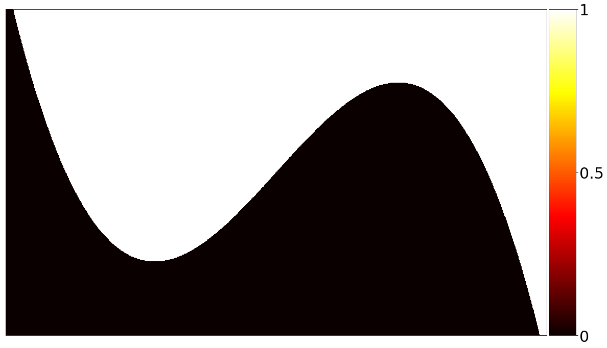
The value of \(\chi\) at each point \(\mathbf r \in \Omega\) is represented by the colors in the color bar on the right. These colors are meant to evoke heat, with white representing large values of \(\chi\) (hot temperatures), black representing low values of \(\chi\) (cold temperatures), and yellow and representing intermediate values.

Diffusion

Now let’s implement the previously described numerical scheme and visualize the diffused characteristic function \(\chi\).

def diffuse(X0, k, hx, hy):
    # Important quantities.
    n, m = X0.shape[0] - 2, X0.shape[1] - 2
    hx_sqinv, hy_sqinv = 1 / hx**2, 1 / hy**2

    # Construct A.
    B_diags = [n * [(2 * hx_sqinv) + (2 * hy_sqinv)], (n-1) * [-hx_sqinv], (n-1) * [-hx_sqinv]]
    B = sp.diags(B_diags, [0, -1, 1])
    C_diags = [(m-1) * [1], (m-1) * [1]]
    C = sp.diags(C_diags, [-1, 1])
    A = sp.kron(sp.eye(m), B) - hy_sqinv * sp.kron(C, sp.eye(n))

    # Boundary conditions.
    b = np.empty(n*m)
    b[:n] = hy_sqinv * X0[1:-1,0]
    print(X0[1:-1,0].shape)
    b[n:-n] = 0
    b[-n:] = hy_sqinv * X0[1:-1,-1]
    temp = np.array(range(b.size))
    b[np.mod(temp, n) == 0] += hx_sqinv * X0[0,1:-1]
    b[np.mod(temp, n) == n - 1] += hx_sqinv * X0[-1,1:-1]

    # Solve linear system and reshape solution, keeping original boundary.
    s = X0[1:-1, 1:-1].reshape((n*m,), order='F') + k * b
    X_temp, _ = splin.cg(sp.eye(n*m) + k * A, s)
    X1 = np.empty(X0.shape, dtype=X0.dtype)
    X1[1:-1,1:-1] = X_temp.reshape((n, m), order='F')
    X1[0,:], X1[-1,:], X1[:,0], X1[:,-1] = X0[0,:], X0[-1,:], X0[:,0], X0[:,-1]

    return X1;

# Diffuse.
chi1 = diffuse(chi0, k, hx, hy)

# Plot.
fig2, ax2 = plt.subplots(figsize=(10, 15))
plot(chi1, ax2, colorbar=True)
plt.show()

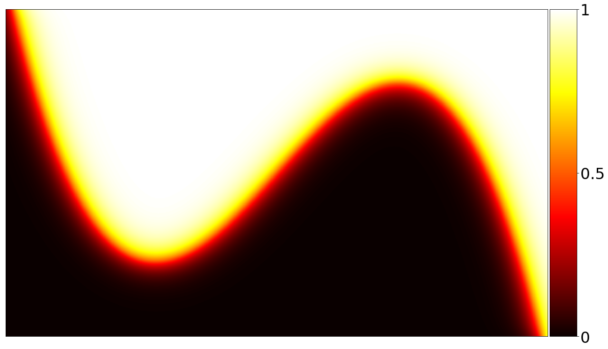
We used a relatively large time step of \(k = 1/250\) to generate a visually appealing image with a wide band of intermediate temperatures (i.e., yellow and red). If we shorten the time step to \(1 / 10000\) and iteratively diffuse \(\chi\), we obtain the following video modeling the evolution of \(\chi\) under the diffusion equation.

Of course, the MBO scheme does not iteratively diffuse \(\chi\) as in the above video, but rather inserts a thresholding step in between each diffusion.

Thresholding

By comparison to the diffusion step, the thresholding step is extremely simple and can be accomplished in a single line of code. In the cell below, we display side-by-side snapshots of \(\Omega\) before and after one iteration of the MBO scheme (i.e., after one diffusion step and subsequent thresholding).

# Threshold.
chi1 = np.round(chi1)

# Plot.
fig3, (ax3, ax4) = plt.subplots(1, 2, figsize=(10,15))
plot(chi0, ax3, colorbar=False)
plot(chi1, ax4, colorbar=False)
ax3.set_title(r"$\Omega$ at initial time.")
ax4.set_title(r"$\Omega$ after one iteration of MBO scheme.")
plt.show()

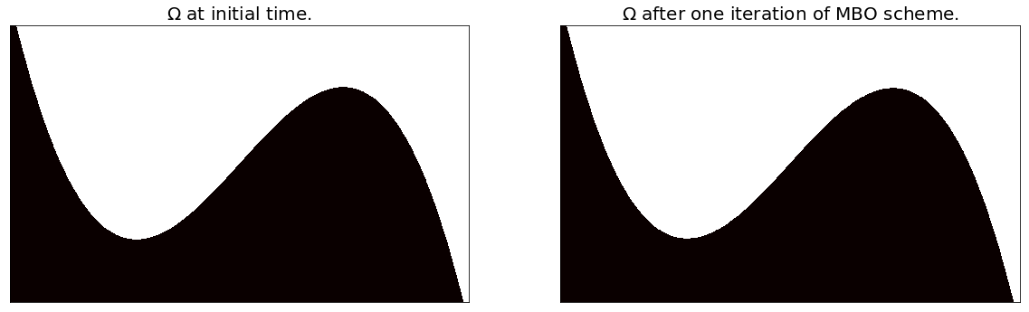
While the above images appear virtually identical, the boundary between black and white has in fact shifted by a few pixels.

Final Product

Using our original time step of \(k = 250\) and iteratively applying the alternating steps of diffusion and thresholding, the MBO scheme produces the following model of mean curvature flow.

And voilà! Motion by mean curvature.

Possible Improvements

The primary bottleneck in the above code is incurred while solving the linear system in \eqref{eq:poisson_system}. In the future, I may implement a fast Poisson solver using the Discrete Sine Transform or a multigrid technique in order to improve performance.

Acknowledgment

I am thankful to Professor Hailong Guo, whose numerical analysis course and office hour discussions enabled me to understand and implement the finite difference method described above.

References

[1] Barry Merriman, James Kenyard Bence, and Stanley Osher. Diffusion Generated Motion by Mean Curvature. Department of Mathematics, University of California, Los Angeles, 1992.

[2] Ekaterina Merkurjev, Tijana Kostic, and Andrea L. Bertozzi. An MBO Scheme on Graphs for Classification and Image Processing. SIAM Journal on Imaging Sciences, 6(4):1903–1930, 2013.

[3] Guy Barles and Christine Georgelin. A Simple Proof of Convergence for an Approximation Scheme for Computing Motions by Mean Curvature. SIAM Journal on Numerical Analysis, 32(2):484–500, 1995.

[4] Lawrence C. Evans. Convergence of an Algorithm for Mean Curvature Motion. Indiana University Mathematics Journal, pages 533–557, 1993.