\(\newcommand{\pagerank}{\mathrm{PageRank}}\newcommand\given[1][]{\:#1\vert\:}\newcommand{\diag}{\mathrm{diag}}\)
NCAARank
This post provides an introduction to PageRank, Google’s algorithm for ranking web pages based upon their link structure. In a nutshell, the algorithm models the behavior of an internet surfer who navigates the web by randomly selecting hyperlinks and occasionally entering URLs. While best known as a method for ranking web sites, PageRank has found a variety of applications beyond the web, including assessing the hydrogen bond potential of a solvent, predicting the flow of traffic or the movement of pedestrians in urban spaces, and identifying influential individuals in a social network [1]. I’ll first introduce the mathematics behind the PageRank algorithm, including a discussion of random walks, Markov chains, and the Perron-Frobenius Theorem. I’ll then use PageRank to produce a ranking of NCAA basketball teams by constructing a so-called “winner network” that models the behavior of a prototypical “bandwagon” fan who frequently shifts his allegiance to follow the best teams.
The Mathematics of PageRank
I’ll introduce the mathematics of PageRank in its original context of ranking web pages. If you’re already familiar with how PageRank works, make sure you understand sink preferential PageRank and then skip to the application section.
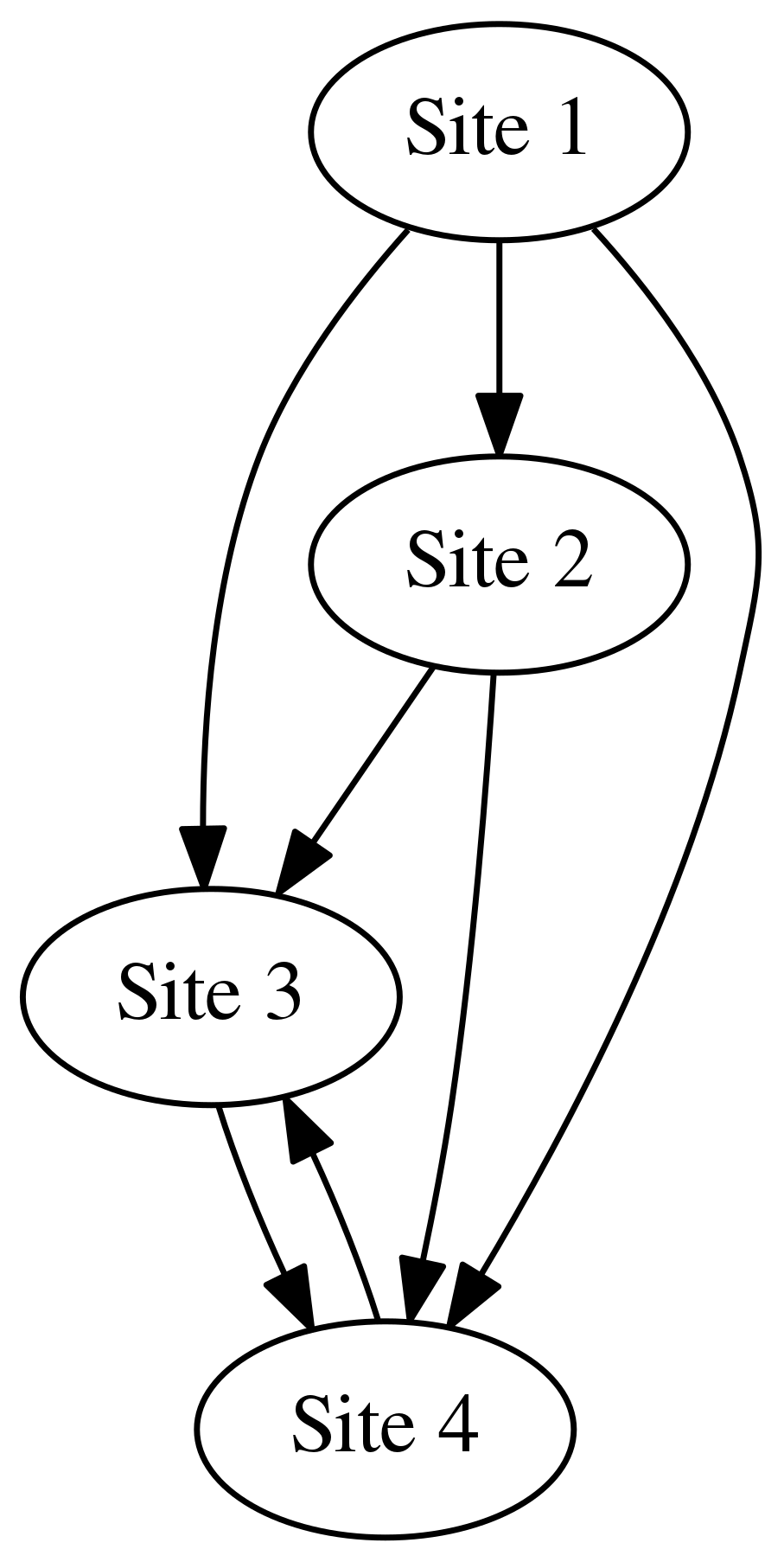
The basic idea of PageRank is to represent the internet as an unweighted directed graph \(G = (V, E)\) in which the vertices of \(V\) represent web pages and the directed edges of \(E\) represent hyperlinks. A random walk on \(G\) models the behavior of a surfer who navigates the web by following hyperlinks uniformly at random and occasionally typing in URLs at random. Such a random walk converges to a unique “stationary distribution,” a probability mass function \(\boldsymbol \pi\) on the vertex set \(V\) that remains unchanged at each step of the random walk. PageRank ranks each web page by the probability that our “random” surfer visits the web page, according to the stationary distribution \(\boldsymbol\pi\).
Random Walks
Let \(G = (V, E)\) with \(\lvert V \rvert = n\) denote the unweighted directed graph described above. The adjacency matrix \(A \in \mathbb R^{n\times n}\) for \(G\) is defined by
\[
a_{ij} =
\begin{cases}
1 &\mbox{if \((i,j) \in E\),}\
0 &\mbox{otherwise}
\end{cases}
\]
for \(1 \leq i \leq n\). That is, \(a_{ij}\) is 1 if there is a hyperlink from web page \(i\) to web page \(j\) and 0 otherwise.
We define the outdegree of a vertex \(i \in V\) by \begin{equation} \label{eq:outdegree} r_i = \sum_{j=1}^n a_{ij}, \end{equation} so that \(r_i\) denotes the number of hyperlinks from webpage \(i\) to other pages. A random walk on \(G\) is a sequence of vertices \((v_t)_{t \geq 0}\) chosen iteratively so that \begin{equation} \label{eq:iterative_pagerank} P(v_{t+1} = j \given v_t = i) = a_{ij} / r_i \end{equation} for all \(i,j\in V\). Intuitively, we can imagine an internet user starting at some initial webpage and surfing the web by clicking on hyperlinks uniformly at random. This suggests a pitfall in our definition, since the graph \(G\) may contain vertices with no outgoing edges corresponding to web pages with no hyperlinks. It is thus possible for our internet surfer to “get stuck” on a so-called “dangling node.” One method of resolving this pitfall is to introduce a so-called “teleportation parameter” \(\alpha\) satisfying \(0 \leq \alpha < 1\) to represent the probability that our internet surfer follows a hyperlink at any given time step (in practice, \(\alpha\) is chosen to be close to 1 so that our surfer almost always follows a hyperlink). However, with probability \(1 - \alpha\), the surfer will type in a URL and “teleport” to a (possibly non-adjacent) vertex chosen uniformly at random from the vertex set \(V\). The probability that an internet user at web page \(i\) at time \(t\) will visit web page \(j\) at time \(t + 1\) is thus given by
\begin{equation} \label{eq:pagerank_transition_probability}
P(v_{t+1} = j \given v_t = i) =
\begin{cases}
\alpha\left(\frac{a_{ij}}{r_i}\right) + \frac{1-\alpha}{n} & \mbox{if \(r_i \neq 0\),} \
\frac 1n & \mbox{otherwise.}
\end{cases}
\end{equation}
The above equation is equivalent to the most common formulation of PageRank, known as strongly preferential PageRank, when used with a uniform teleportation distribution. Later in this post, I’ll introduce a more general framework for understanding PageRank and will explain a few less common versions of the algorithm.
Markov Chains and the Perron-Frobenius Theorem
The random walk described above is an example of a Markov chain, a stochastic model of a sequence of random events in which the probability that the next event occurs is determined solely by the current event. For example, the probability that a random walk on \(G\) will visit some vertex at the next time step depends only on the current vertex, not on previously visited vertices. Markov chains on a finite set of events may be described using Markov matrices (also known as stochastic matrices), real square matrices with non-negative entries such that each row sums to 1. The entry \(m_{ij}\) of a Markov matrix \(M\) indicates the probability that a random walker located at vertex \(i\) at time \(t\) moves to vertex \(j\) at time \(t + 1\). A probability distribution on the vertex set \(V\) may be represented as a stochastic vector, a row vector with real, non-negative entries that sum to 1. If \(M \in \mathbb R^{n \times n}\) is a Markov matrix for a random walk on the graph \(G\) and \(\mathbf p^0 \in \mathbb R^{1 \times n}\) is a stochastic vector such that \(\mathbf p^0_i\) indicates the probability that the random walk starts at vertex \(i\), you can verify that \(\mathbf p^1 = \mathbf p^0M\) is a stochastic vector in which \(\mathbf p^1_j\) denotes the probability that the random walker is located at vertex \(j\) after one time step. By induction, \(\mathbf p^s = \mathbf p^0M^s\) is then a stochastic vector in which \(\mathbf p^s_i\) denotes the probability that the random walker is located at vertex \(i\) after \(s\) time steps.
We can conveniently represent the random walk of our internet surfer by the Markov matrix \(M \in \mathbb R^{n \times n}\), where \(m_{ij}\) denotes the probability defined in \eqref{eq:pagerank_transition_probability}. In virtue of the positive teleportation parameter \(\alpha\), this matrix has the special property of being a positive matrix (i.e., \(m_{ij} > 0\) for \(1 \leq i, j \leq n\)). \(M\) thus satisfies the conditions of the Perron-Frobenius Theorem as presented below. I must introduce a few definitions to state this theorem precisely. First, a real vector is said to be positive if each of its entries is positive. Second, an eigenvalue \(\lambda\) associated to the matrix \(A \in \mathbb C^{n \times n}\) is said to be dominant if it has multiplicity 1 and its modulus is strictly greater than the modulus of any other eigenvalue. The eigenvector of \(A\) corresponding to \(\lambda\) is called the dominant eigenvector of \(A\).
(Note: I haven’t stated the Perron-Frobenius Theorem in full generality, but this version will suffice for our current purposes.) Since \(M\) is a Markov matrix, \(M\mathbf 1 = \mathbf 1\), where \(\mathbf 1 \in \mathbb R^n\) denotes the one-vector whose entries are all 1. Now \(M\) is a positive matrix and \(\mathbf 1\) is a positive right eigenvector of \(M\) corresponding to \(\lambda = 1\), so the Perron-Frobenius Theorem implies that \(1\) is the dominant eigenvalue of \(M\) and that there exists a unique positive left eigenvector \(\boldsymbol \pi\) of \(M\) corresponding to \(\lambda = 1\) such that \(\lVert \boldsymbol \pi \rVert_1 = 1\). \(\boldsymbol \pi\) is the unique stochastic vector satisfying \(\boldsymbol \pi M = \boldsymbol \pi\), and is thus known as the stationary distribution associated to the Markov matrix \(M\), since it remains unchanged at each time step of the random walk. By the final statement of the Perron-Frobenius Theorem, \[ \lim_{k\rightarrow \infty} M^k = \mathbf 1 \boldsymbol \pi. \] For any stochastic vector \(\mathbf p_0 \in \mathbb R^{1 \times n}\) representing an initial probability distribution on the vertex set \(V\), we can left-multiply the above equation by \(\mathbf p_0\) to obtain \[ \lim_{k\rightarrow\infty} \mathbf p_0M^k = \boldsymbol \pi. \] Intuitively, this equation states that any initial probability distribution converges to the stationary distribution \(\boldsymbol \pi\). We then define the PageRank as a real-valued function on the vertex set \(V\), \[ \pagerank(i) = \boldsymbol \pi_i, \quad i \in V. \] In other words, the PageRank of a webpage \(i\) is the probability that a surfer visits the webpage \(i\), according to the stationary distribution \(\boldsymbol \pi\). Pages for which this probability is high are deemed important, and a ranking of the relative importance of all pages on the web may be obtained by sorting the entries of \(\boldsymbol \pi\).
A More General Framework
As promised, I’ll now present a more general framework for PageRank that will allow me to discuss three variants on the algorithm as presented in [2]. Suppose we start with a directed graph \(G\) and try to construct a Markov matrix for a random walk on the graph. However, we reach a dangling node and are dismayed to find that an entire row of our matrix \(\overline P\) is zero. This failed stochastic matrix is an example of a substochastic matrix, a square matrix with non-negative entries and rows that sum to at most 1. A random walk on \(G\) is ill-defined, since our random walker does not know where to go when he reaches a dangling node. To remedy this issue, we fix all the dangling nodes by adding outgoing edges, or equivalently, by changing the rows of zeros in \(\overline P\) to obtain a fully stochastic matrix \(P\). However, the geometric multiplicity of the eigenvalue 1 of a stochastic matrix may be greater than 1 (for example, if \(P\) is a permutation matrix). Thus, the dominant eigenvector of \(P\) may fail to be unique. PageRank resolves this issue by constructing the positive Markov matrix \begin{equation} \label{eq:positive_markov} M = \alpha P + (1 - \alpha) \mathbf 1 \mathbf v, \end{equation} where \(0 \leq \alpha < 1\) is the aforementioned “teleportation parameter” and \(\mathbf v \in \mathbb R^{1 \times n}\) is a stochastic vector known as the “teleportation distribution.” As its name suggests, \(\mathbf v\) describes how a random walker should behave when he “teleports” rather than following the edges of the graph. The core PageRank problem is then the eigenvalue problem \[ \mathbf x M = \mathbf x \qquad \mbox{subject to} \quad \lVert \mathbf x \rVert_1 = 1, \quad \mathbf x > 0, \] which is guaranteed to have a unique solution by the Perron-Frobenius Theorem. (Note: If \(\mathbf v\) is a non-positive stochastic vector, then the Markov matrix \(M\) may be non-positive and the Perron-Frobenius theorem may not apply. It turns out that the stationary distribution is still unique in such a case, and so non-positive teleportation distributions are permitted. See [2] for a discussion.) The three versions of PageRank I will discuss, known as strongly preferential, weakly preferential, and sink preferential, all follow this general framework and differ only in how the stochastic matrix \(P\) is constructed from the substochastic matrix \(\overline P\).
The strongly preferential rendition of PageRank is common enough that it is sometimes referred to as the PageRank algorithm. Let \(\mathbf d\in\mathbb R^n\), where \(\mathbf d_i = 1\) if the ith row of \(\overline P\) contains only zeros, and \(\mathbf d_i = 0\) otherwise. Strongly preferential PageRank starts with the substochastic matrix \(\overline P\) and then constructs the stochastic matrix \(P_{\mathbf v} := \overline P + \mathbf d\mathbf v\), where \(\mathbf v \in \mathbb R^{1 \times n}\) is importantly the same teleportation distribution as in \eqref{eq:positive_markov}. In other words, \(P_{\mathbf v}\) is obtained by replacing all rows of zeros in \(\overline P\) by the teleportation distribution \(\mathbf v\), allowing a random walker to escape from any dangling node. You can verify that if \(\mathbf v\) is chosen to be the uniform distribution (i.e., \((1 / n)\mathbf 1^T\)), then the (i, j)th entry of \(M = \alpha P_{\mathbf v} + (1 - \alpha) \mathbf 1 \mathbf v\) is equal to \eqref{eq:pagerank_transition_probability}.
Weakly preferential PageRank differs from the strongly preferential variant by relaxing the requirement that the teleportation distribution \(\mathbf v\) be added to the rows of zeros in \(\overline P\). It instead defines \(P_{\mathbf u} := \overline P + \mathbf d \mathbf u\) for some stochastic vector \(\mathbf u \in \mathbb R^{1\times n}\) that is independent of \(\mathbf v\). This rendition of PageRank might be preferable if we have some intuition of how our random walker should behave when he encounters a dangling node. The last version of PageRank, known as sink preferential PageRank, is perhaps the simplest. In this version, a random walker simply stays put when he encounters a dangling node. Mathematically, a self-loop is added to each dangling node, and the stochastic matrix for the random walk is defined as \(P_{\mathbf d} = \overline P + \diag(\mathbf d)\). As I’ll now explain, the sink preferential version of PageRank is best suited for the task of ranking NCAA tournament teams.
March Madness Power Ranking
Each year, 32 college teams automatically qualify for the NCAA men’s basketball tournament, and an additional 36 teams are selected by a committee of experts. All 68 teams are then ranked in a seeding process that determines 60 of the 64 slots in the NCAA bracket, with the eight lowest-seeded teams competing in four games to qualify for the remaining four slots. Let’s take a moment to appreciate the difficulty of accurately and fairly ranking these teams. As of this writing, there are 351 Division I men’s basketball programs, but a typical regular season consists of only about 30 games. It is thus a mathematical certainty that the vast majority of teams will never face each other during the course of a single regular season. Moreover, strength of schedule can vary widely between different conferences. For example, the Atlantic Coast Conference (ACC), which sent nine teams to the 2018 NCAA tournament, is vastly more competitive than the Pac-12, which sent only three. Thus, a naive comparison of records, point differentials, or other in-game statistics will inevitably penalize worthy teams who simply play against stiffer competition. As we shall see, the PageRank algorithm is well-suited to precisely this type of problem, since it was designed for sparse graphs and automatically adjusts for strength of schedule.
The Winner Network
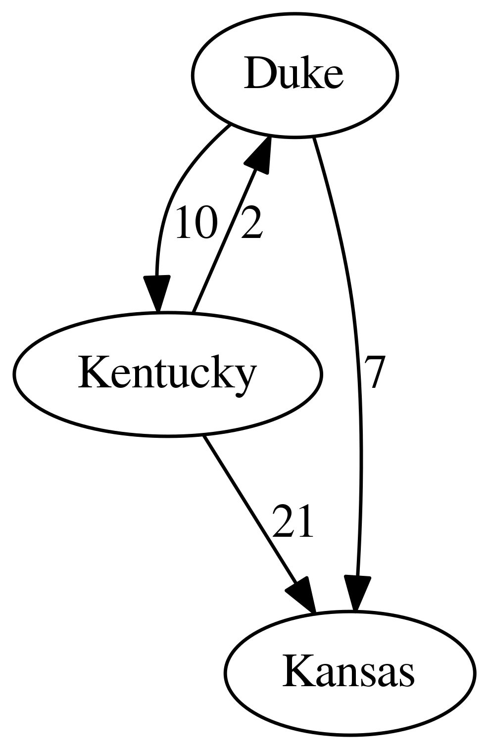
Applying PageRank supposes we have constructed some sort of graph to represent our data. In the current context, we’ll construct a so-called “winner network,” a graph whose vertices represent teams and whose edges describe the flow of “prestige” from one team to another. After each game, a directed edge from the loser to the winner will be added to the graph and weighted by the margin of victory (in contrast to the unweighted graph representing the internet). If two teams face each other a second time, we simply add the margin of victory to the appropriate edge.
If \(w_{ij}\) denotes the weight of the edge from \(i\) to \(j\), the outdegree of node \(i\) in the weighted graph \(G\) is the same as \eqref{eq:outdegree} (replacing \(a_{ij}\) by \(w_{ij}\)), and a random walk on \(G\) is an iteratively chosen sequence of vertices satisfying \eqref{eq:iterative_pagerank} (replacing \(a_{ij}\) by \(w_{ij}\)). A random walk on the winner network has the attractive interpretation of a bandwagon fan who randomly changes his loyalty based upon the fortunes of his current team. The winner network and strongly preferential PageRank have been used in [3] and [4] to rank NFL teams and professional tennis players, respectively. In contrast to these rankings, I elect to use the sink preferential variant of PageRank. As noted in [1], sink preferential PageRank has an intuitive justification in the context of the winner network, since dangling nodes represent undefeated teams that the prototypical bandwagon fan would be unlikely to abandon.
Data Set and Implementation
I used Python’s urllib and BeautifulSoup packages to visit individual team pages on Sports Reference and scrape game statistics for the 2017-18 season. Let’s load the data set and display the first five regular season Duke games.
import pandas as pd
import numpy as np
import scipy.sparse.linalg as splin
from IPython.display import display, HTML

# Load DataFrame.
path = 'data/2017-18/'
file = 'scores.csv'
df = pd.read_csv(path + file, index_col=0, parse_dates=['Date'])

# Display first five Duke games.
team = 'duke'
ind = (df['Team1']==team) | (df['Team2']==team)
display(HTML(df.loc[ind].head().to_html(index=False)))
| Date | GameType | Team1 | Pts1 | Team2 | Pts2 |
|---|---|---|---|---|---|
| 2017-11-10 | REG | duke | 97 | elon | 68 |
| 2017-11-11 | REG | duke | 99 | utah-valley | 69 |
| 2017-11-14 | REG | duke | 88 | michigan-state | 81 |
| 2017-11-17 | REG | duke | 78 | southern | 61 |
| 2017-11-20 | REG | duke | 92 | furman | 63 |
Some statistics will give us a better idea of the contents of our data set.
# List of teams.
teams = df['Team1'].values.tolist() + df['Team2'].values.tolist()
teams = list(set(teams))
teams.sort()
n = len(teams)

# Pre-tournament DataFrame.
pre_df = df[df['Date'] < '2018-03-13']
pre_df = pre_df.drop(['Date', 'GameType'], axis=1)

# NCAA tournament DataFrame.
tourn_df = df[df['GameType']=='NCAA']
tourn_df = tourn_df.drop(['GameType'], axis=1)

# Display stats.
index = [ 'Teams', 'Total Games', 'Pre-tournament Games', 'Tournament Games' ]
data = [ n, len(df.index), len(pre_df.index), len(tourn_df.index) ]
columns = [ 'Category', 'Count']
stats_df = pd.DataFrame(list(zip(index, data)), columns=columns)
stats_df = stats_df.set_index('Category')
display(stats_df)
| Count | |
|---|---|
| Category | |
| Teams | 656 |
| Total Games | 6004 |
| Pre-tournament Games | 5874 |
| Tournament Games | 67 |
Our data set contains 6004 games played between 656 NCAA teams from Division I, II, and III in the 2017-18 season. The NCAA tournament itself consists of 67 games between 68 teams: four qualification games and 63 elimination games in a bracket of 64 teams. I’ll use sink preferential PageRank to rank all 656 teams based upon their performance prior to the start of the 2018 NCAA men’s basketball tournament on March 13. I’ll then use the outcome of the tournament games to evaluate PageRank relative to other rankings.
Now comes the actual implementation of PageRank. As mentioned previously, I have elected to use the sink preferential construction of the positive Markov matrix \(M\) with a uniform teleportation distribution. In keeping with [3], I set the teleportation parameter to \(\alpha = 0.85\).
# Create a dictionary mapping team names to indices.
team_dict = dict(zip(teams, range(n)))

# Sub-stochastic matrix P_bar.
P_bar = np.zeros((n, n))

# Add an edge from loser to winner with margin of victory as edge weight.
for _, row in pre_df.iterrows():
    team1, pts1, team2, pts2 = row.values.tolist()
    sorted_tuples = sorted([(team1, pts1), (team2, pts2)], key=lambda tuple: tuple[1])
    i, j = [ team_dict[tuple[0]] for tuple in sorted_tuples ]
    P_bar[i,j] += abs(pts1 - pts2)

# Make nonzero rows sum to 1. Now P_bar is sub-stochastic.
row_sum = P_bar.sum(axis=1, dtype='float64')
d = row_sum==0
temp_ind = ~d
inv_row_sum = np.zeros(row_sum.shape)
inv_row_sum[temp_ind] = np.reciprocal(row_sum[temp_ind])
P_bar = P_bar * inv_row_sum[:, np.newaxis]

# Stochastic Markov matrix P for sink preferential PageRank.
P = P_bar + np.diag(d)

# Teleportation parameter alpha.
alpha = 0.85

# Positive Markov matrix M with uniform teleportation distribution.
M = alpha * P + (1 - alpha) * (1 / n)
Now that I’ve constructed \(M\), the next step is find the dominant eigenvector and stationary distribution \(\boldsymbol\pi\).
# Solve for dominant eigenvector of M and normalize.
_, pi = splin.eigs(M.T, k=1)
pi = np.real(pi.squeeze())
pi = pi / np.sum(pi)

# Display most highly ranked teams.
tuples = zip(teams, pi.tolist())
tuples = sorted(tuples, key=lambda tuple: tuple[1], reverse=True)
columns = [ 'Team', 'PageRank' ]
pr_df = pd.DataFrame(tuples, columns=columns)
pr_df = pr_df.set_index('Team')
display(pr_df.head(25))
| PageRank | |
|---|---|
| Team | |
| villanova | 0.024310 |
| west-virginia | 0.021227 |
| kansas | 0.015281 |
| virginia | 0.013761 |
| butler | 0.013637 |
| north-carolina | 0.013312 |
| alabama | 0.013008 |
| xavier | 0.012924 |
| florida | 0.012778 |
| michigan | 0.012000 |
| duke | 0.011624 |
| creighton | 0.011369 |
| texas-am | 0.011353 |
| providence | 0.011131 |
| texas-tech | 0.010611 |
| kentucky | 0.010300 |
| auburn | 0.009923 |
| houston | 0.009698 |
| tennessee | 0.009612 |
| purdue | 0.009551 |
| michigan-state | 0.009412 |
| gonzaga | 0.008738 |
| ohio-state | 0.008433 |
| cincinnati | 0.008282 |
| texas-christian | 0.008100 |
The above table includes the PageRank of the 25 most highly ranked teams. It’s notable that PageRank rated Villanova, the eventual winner of the 2018 NCAA tournament, as the best team in college basketball. According to the stationary distribution \(\boldsymbol\pi\), a random fan has a 2.4% chance of rooting for Villanova – quite a high percentage when one considers that the ranking includes 656 teams.
To evaluate PageRank, I’ll first compare its predictive accuracy in tournament games to rankings from Bleacher Report, 538, and the official NCAA list used to seed the tournament. These rankings include all 68 teams and were compiled shortly before the start of the tournament. The data has been cleaned and stored in a .csv file.
# Load rankings.
file = 'ranking.csv'
ranking_df = pd.read_csv(path + file, index_col=0)

# Add PageRank ranking for tournament teams.
tourn_teams = ranking_df.index.tolist()
pr_dict = pr_df.to_dict()['PageRank']
pr = [ pr_dict[team] for team in tourn_teams ]
tuples = zip(tourn_teams, pr)
tuples = sorted(tuples, key=lambda tuple: tuple[1], reverse=True)
pr_teams, _ = zip(*tuples)
pr_dict = dict(zip(pr_teams, range(1, 70)))
ranking_df['PageRank'] = pd.Series(pr_dict)
with pd.option_context('display.max_rows', None):
    display(ranking_df)
| BR | 538 | Seed | PageRank | |
|---|---|---|---|---|
| Team | ||||
| alabama | 23 | 35 | 36 | 7 |
| arizona | 8 | 15 | 16 | 32 |
| arizona-state | 36 | 45 | 43 | 26 |
| arkansas | 30 | 31 | 26 | 30 |
| auburn | 25 | 25 | 13 | 17 |
| bucknell | 55 | 51 | 55 | 60 |
| buffalo | 53 | 48 | 51 | 54 |
| butler | 45 | 23 | 33 | 5 |
| cal-state-fullerton | 63 | 63 | 61 | 64 |
| cincinnati | 14 | 6 | 8 | 24 |
| clemson | 19 | 24 | 19 | 35 |
| college-of-charleston | 56 | 55 | 53 | 57 |
| creighton | 37 | 30 | 30 | 12 |
| davidson | 47 | 37 | 48 | 50 |
| duke | 3 | 3 | 6 | 11 |
| florida | 20 | 18 | 21 | 9 |
| florida-state | 50 | 27 | 38 | 41 |
| georgia-state | 58 | 56 | 60 | 52 |
| gonzaga | 12 | 9 | 15 | 22 |
| houston | 17 | 19 | 23 | 18 |
| iona | 61 | 59 | 62 | 65 |
| kansas | 5 | 7 | 3 | 3 |
| kansas-state | 33 | 42 | 34 | 39 |
| kentucky | 9 | 13 | 17 | 16 |
| lipscomb | 65 | 62 | 59 | 58 |
| long-island-university | 67 | 67 | 66 | 67 |
| loyola-il | 48 | 43 | 46 | 42 |
| marshall | 43 | 57 | 54 | 47 |
| maryland-baltimore-county | 62 | 64 | 63 | 62 |
| miami-fl | 27 | 26 | 22 | 45 |
| michigan | 10 | 12 | 11 | 10 |
| michigan-state | 4 | 4 | 9 | 21 |
| missouri | 21 | 50 | 32 | 38 |
| montana | 54 | 54 | 56 | 55 |
| murray-state | 49 | 49 | 50 | 51 |
| nevada | 39 | 39 | 27 | 36 |
| new-mexico-state | 44 | 47 | 47 | 49 |
| north-carolina | 7 | 8 | 5 | 6 |
| north-carolina-central | 68 | 68 | 67 | 66 |
| north-carolina-greensboro | 57 | 53 | 52 | 48 |
| north-carolina-state | 34 | 40 | 37 | 29 |
| ohio-state | 29 | 20 | 20 | 23 |
| oklahoma | 40 | 36 | 40 | 28 |
| pennsylvania | 60 | 58 | 64 | 63 |
| providence | 28 | 44 | 35 | 14 |
| purdue | 11 | 5 | 7 | 20 |
| radford | 66 | 65 | 65 | 59 |
| rhode-island | 24 | 33 | 28 | 43 |
| san-diego-state | 38 | 41 | 45 | 33 |
| seton-hall | 22 | 21 | 29 | 37 |
| south-dakota-state | 42 | 52 | 49 | 44 |
| st-bonaventure | 32 | 46 | 42 | 53 |
| stephen-f-austin | 52 | 60 | 58 | 56 |
| syracuse | 51 | 38 | 44 | 46 |
| tennessee | 13 | 17 | 10 | 19 |
| texas | 46 | 34 | 39 | 31 |
| texas-am | 31 | 28 | 25 | 13 |
| texas-christian | 41 | 22 | 24 | 25 |
| texas-southern | 64 | 66 | 68 | 68 |
| texas-tech | 16 | 16 | 12 | 15 |
| ucla | 26 | 32 | 41 | 40 |
| villanova | 1 | 1 | 2 | 1 |
| virginia | 2 | 2 | 1 | 4 |
| virginia-tech | 35 | 29 | 31 | 34 |
| west-virginia | 15 | 11 | 18 | 2 |
| wichita-state | 18 | 14 | 14 | 27 |
| wright-state | 59 | 61 | 57 | 61 |
| xavier | 6 | 10 | 4 | 8 |
The table above shows all four rankings of the 68 tournament teams. In addition to the above rankings, I also found archived decimal odds for each tournament game from Odds Portal. While these odds do not represent rankings per se, they nonetheless provide a meaningful benchmark of predictive accuracy.
# Load and display odds.
file = 'odds.csv'
odds_df = pd.read_csv(path + file, index_col=0)
tourn_df = pd.merge(tourn_df, odds_df, on=['Team1', 'Team2'])
display(HTML(tourn_df.head().to_html(index=False)))
| Date | Team1 | Pts1 | Team2 | Pts2 | Odds1 | Odds2 |
|---|---|---|---|---|---|---|
| 2018-03-13 | long-island-university | 61 | radford | 71 | 3.01 | 1.41 |
| 2018-03-13 | st-bonaventure | 65 | ucla | 58 | 2.27 | 1.67 |
| 2018-03-14 | arizona-state | 56 | syracuse | 60 | 1.85 | 1.99 |
| 2018-03-14 | north-carolina-central | 46 | texas-southern | 64 | 2.93 | 1.43 |
| 2018-03-15 | michigan | 61 | montana | 47 | 1.16 | 5.53 |
Decimal odds represent the return on a successful $1 bet. For example, in the last game in the above table, a successful $1 bet on Michigan would earn $1.16 (for a $0.16 profit) while a successful $1 bet on Montana would earn $5.53 (for a $4.53 profit). The team with the lower decimal odds (in this case, Michigan) is considered the favorite.
I’ll now compare rankings by counting the number of correctly predicted games, i.e., the number of games in which the higher ranked team won. I’ll also count the number of tournament games correctly predicted by Vegas, i.e., the number of games in which the favorite won.
# Index with True if team 1 won, False otherwise.
win_ind = tourn_df['Pts1'] > tourn_df['Pts2']

# Team lists.
cols = [ 'Team1', 'Team2' ]
teams1, teams2 = [ tourn_df[col].tolist() for col in cols ]

# Rankings.
data = list()
for col, rank_dict in ranking_df.to_dict().items():
    rank1 = np.array([ rank_dict[team] for team in teams1 ])
    rank2 = np.array([ rank_dict[team] for team in teams2 ])
    ind = rank1 < rank2
    data.append([col, sum(win_ind==ind)])

# Odds.
odds_ind = tourn_df['Odds1'] < tourn_df['Odds2']
data.append([ 'Vegas Odds', sum(win_ind==odds_ind) ])

columns = [ 'Ranking', 'Corr. Pred.' ]
comp_df = pd.DataFrame(data, columns=columns)
comp_df = comp_df.set_index('Ranking')
comp_df['Accuracy'] = comp_df['Corr. Pred.'] / 68
comp_df = comp_df.sort_values('Corr. Pred.', ascending=False)
display(comp_df)
| Corr. Pred. | Accuracy | |
|---|---|---|
| Ranking | ||
| 538 | 47 | 0.691176 |
| BR | 46 | 0.676471 |
| Vegas Odds | 45 | 0.661765 |
| Seed | 44 | 0.647059 |
| PageRank | 43 | 0.632353 |
A strategy of random guessing would result in an expected value of \(\mu = 33.5\) correct predictions with standard deviation \(\sigma \approx 4.09\). The observed number of 43 correct predictions for PageRank lies roughly 2.3 standard deviations above the mean and is statistically significant at the 0.05 level. From the (admittedly small) sample of the 2018 NCAA men’s tournament, it appears that PageRank is competitive with the other tournament rankings. It underperforms the other rankings by only a narrow margin, falling short of the official seed ranking by a single game. This feat is perhaps more impressive when one considers that PageRank uses only a single game statistic, margin of victory, to produce its ranking. In contrast, the most accurate ranking from 538 employs a sophisticated ensemble of models. I thus conclude that PageRank provides a reasonable “first-order approximation” to the true ranking of NCAA teams, one that could perhaps be improved by incorporating a richer set of features or using PageRank in tandem with other models.
References
[1] David Francis Gleich. PageRank Beyond the Web. SIAM Review, 57(3):321–363, 2015.
[2] David Francis Gleich. Models and Algorithms for PageRank Sensitivity. Ph.D. thesis, Stanford University, 2009.
[3] Anjela Y Govan, Carl D Meyer, and Russell Albright. Generalizing Google’s PageRank to Rank National Football League Teams. In Proceedings of the SAS Global Forum, Volume 2008, 2008.
[4] Filippo Radicchi. Who is the Best Player Ever? A Complex Network Analysis of the History of Professional Tennis. PloS One, 6(2):e17249, 2011.