1000 Genomes: Part I

This post discusses the linear and non-linear dimensionality reduction techniques of dual and kernel PCA in the context of genomic data. I’ll first describe the mathematics behind these techniques (basically, the mathematics of the so-called “kernel trick”) and will then apply them to visualize high-dimensional genomic data in two and three dimensions. The resulting low dimensional representations preserve a great deal of the structure of the original data; for example, distinct gender, ethnic, and racial groups appear as discernible clusters, while groups of mixed heritage are situated in intermediate positions between “parent” populations. In the next post, I’ll use SVMs and neural networks to predict an individual’s ethnic background based on his or her genome.

Previous Work

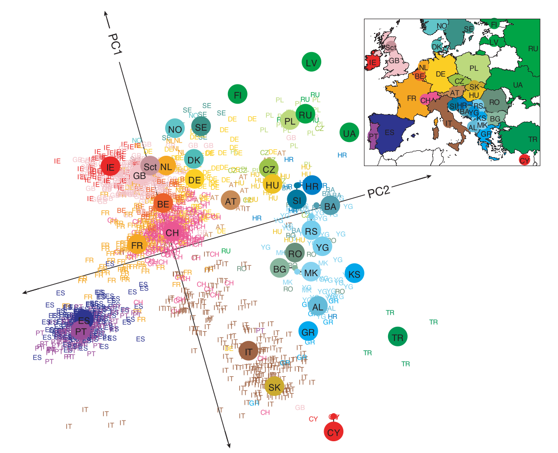
This post was inspired by the most fascinating application of PCA I have yet to encounter, a 2009 study which studied the genomes of 3,192 European individuals at 500,568 loci [1]. Remarkably, a PCA of the genomic data using the top two principal component resulted in a high-resolution map of Europe, reproducing geographic features such as the Iberian and Italian peninsulas and the British Isles, and even resolving sub-populations within individual countries (see Figure 1 below).

Figure 1: A PCA of European genomic data using the top two principal components results in a map of the European subcontinent (image from [1]).

The data set used in the study is unfortunately not publicly available. However, Amazon Web Services hosts the 1000 Genomes Project, containing genomes sequenced at roughly 81 million loci from 2504 individuals belonging to 26 population groups, as a publicly available S3 Bucket. The high dimension of the feature space (in this case, the number of sequenced loci) precludes the possibility of applying standard techniques to compute a PCA of the data. Others have applied more sophisticated techniques to compute a PCA for the data set; for example, [2] uses IRLBA, an efficient algorithm for computing truncated SVDs of large matrices. I will instead use the simpler method of dual PCA in addition to the non-linear method of kernel PCA to reduce the dimension of the data and visualize it in two and three dimensions.

Data Set

The 1000 Genomes Project was an international effort commencing in 2008 and completed in 2015 to catalog human genetic variation. The project sequenced the genomes of 2504 individuals from 26 different population groups from around the world, and the resulting data set was made publicly available for the benefit of future research. Since different individuals share the vast majority of their genomes in common, genomic data is stored in “variant call format” (VCF), which records the differences between individual genomes and a reference genome. Each genome in the study was sampled at roughly 81 million “variant” sites (i.e., sites that frequently differ from the reference genome), resulting in a high-dimensional feature space. Variants may range in length from “single-nucleotide polymorphisms” (SNPs), indicating a change in a single base pair, to several base pairs in length. To illustrate VCF, here’s a small excerpt consisting of two rows from a VCF file from the 1000 Genomes Project (for clarity, I have omitted most columns and have formatted the text so that columns are properly aligned).

#CHROM  POS     REF     ALT     HG00096 HG00097 HG00099 HG00100 HG00101
1       10177   A       AC      1|0     0|1     0|1     1|0     0|0

The second row above corresponds to a variant site located in the first chromosome at position 10177. The reference genome has adenine at this site, while certain individuals have both adenine and cytosine. Identification codes uniquely identify each individual in the study (e.g., “HG00096”). Below these ID codes, the digits to the left and right of the pipe signify whether the reference or alternate sequence are present on the left and right alleles of the corresponding sample, with zero corresponding to the reference sequence and one corresponding to the alternate sequence. For example, sample HG00096 has the variant AC on the left allele and the reference sequence A on the right allele at position 10177 of the first chromosome. In certain cases (not shown above), multiple alternate sequences may be given, in which case positive digits indicate which variant is present. This format applies for chromosomes 1 through 21 and the X chromosome. Since human beings possess at most one allele for the Y chromosome, the VCF entries for this chromosome consist of single digits rather than digits separated by a pipe. In rare cases, a period indicates that data is missing for a particular sample and site.

Processing the Data Set

By recording the sites at which an individual genome differs from the reference genome, variant call format takes advantage of the highly redundant nature of the human genome and lends itself naturally to a sparse matrix representation of the data. For each chromosome, I downloaded the corresponding VCF file from the 1000 Genomes S3 Bucket to an EC2 instance. I then parsed the file with a simple C program that iterates over positions in the genome and individual samples. At each position and for each individual, I ignored which particular variant occurred, instead recording only whether a variant occurred at all. For example, the data for the first chromosome is stored across multiple sparse matrices. Each matrix has 2504 rows corresponding to the samples in the data set, and the combined number of columns is just the number of variant sites in the first chromosome. The (i, j)^th entry of a matrix is 0 if the i^th sample matches the reference genome (on both alleles) at the variant site corresponding to the j^th column, and 1 if a variant occurs. This format is relatively space efficient, since the sparse matrices have Boolean rather than integer entries. Even so, the genomes of all 2504 individuals required roughly eight gigabytes of compressed sparse matrices.

Both of the dimensionality reduction techniques I apply in this post may be implemented using a pairwise distance matrix, so I compute this matrix first. Since the data is binary, Manhattan distance is the same as squared Euclidean distance, i.e., \(\lVert \mathbf x - \mathbf y \rVert_1 = \lVert \mathbf x - \mathbf y \rVert_2^2\) for all samples \(\mathbf x\) and \(\mathbf y\). The Manhattan distance between two genomes has an attractive interpretation in the current context; it simply counts the number of sites at which one genome has the reference sequence of base pairs and the other genome has a variant. Moreover, since Manhattan distance and squared Euclidean distance are equal, we can efficiently compute the Manhattan pairwise distance matrix for each sparse matrix containing a portion of the data set using a vectorized implementation like the one found here. Finally, the pairwise distance matrix for the entire data set can be easily computed by summing the pairwise distance matrices corresponding to each constituent sparse matrix.

Dimensionality Reduction and Data Visualization

With the pairwise distance matrix in hand, we can proceed with our discussion of dual and kernel PCA. The explanation of these techniques provided below assumes a familiarity with principal component analysis, singular value decomposition, and eigendecomposition.

Dual PCA

Suppose a data set \(\mathcal X\) is represented by the matrix \(X \in \mathbb R^{m \times n}\), where \(m\) is the number of samples in the data set and \(n\) is the dimension of the feature space. To compute a standard PCA, we first center the data to obtain the matrix \(X_c\) with column means equal to zero. The principal components of the data are the right eigenvectors of the sample covariance matrix \(\frac{1}{m-1}X_c^T X_c \in \mathbb R^{n \times n}\), or equivalently, the right singular vectors of \(X_c\). The projection of the data onto the top \(k\) principal components is given by \begin{equation} \label{eq:pca_proj} U_k \Sigma_k = X_c V_k, \end{equation} where \(\Sigma \in \mathbb R^{k \times k}\) is the diagonal matrix containing the top \(k\) singular values of \(X_c\) in descending order, \(U_k \in \mathbb R^{m \times k}\) is the matrix of corresponding left singular vectors, and \(V_k\) is the matrix of the top \(k\) principal components. Thus, PCA can be computed using either the singular value decomposition of \(X_c\) or the eigendecomposition of \(X_c^T X_c\).

In the current context, the number of features \(n \approx 81\) million far exceeds the number of samples \(m = 2504\). Due to the high dimension of the feature space, the techniques described above fail since we cannot explicitly compute the sample covariance matrix (let alone its eigendecomposition), nor can we compute the SVD of \(X_c\) using standard techniques. Since the number of samples \(m = 2504\) is relatively modest, we can instead use dual PCA, which essentially amounts to applying the so-called “kernel trick” with a linear kernel. Let’s consider the relatively small Gram matrix for the linear kernel \(X_c X_c^T \in \mathbb R^{m \times m}\) (more on kernels in the next section). If the SVD of \(X_c\) is given by \(X_c = U \Sigma V^T\) for unitary matrices \(U \in \mathbb R^{m \times m}\) and \(V \in \mathbb R^{n \times n}\) and diagonal matrix \(\Sigma \in \mathbb R^{m \times n}\), then the Gram matrix is \[ X_c X_c^T = U \hat{\Sigma}^2 U^T, \] where \(\hat{\Sigma}^2 \in \mathbb R^{m \times m}\) consists of the first \(m\) columns of \(\Sigma\). In other words, we can recover the singular values and left singular vectors in \eqref{eq:pca_proj} by computing the eigendecomposition of the Gram matrix.

There’s one additional caveat. In the current case, we cannot form \(X_c\) since explicitly centering the data in \(X\) would destroy its sparse structure. Fortunately, I’ve already computed the pairwise squared Euclidean distance matrix \(D_{\mathrm{sq}}\) for \(X\). We can easily compute the Gram matrix with the formula \[ X_c X_c^T = -\left(I_m - \dfrac{\mathbf{1}_m \mathbf{1}_m^T}{m}\right) \frac{D_{\mathrm{sq}}}{2} \left(I_m - \dfrac{\mathbf{1}_m \mathbf{1}_m^T}{m}\right), \] where \(\mathbf{1}_m \in \mathbb R^m\) denotes the one-vector whose entries are all one, and the outer product \(\mathbf{1}_m \mathbf{1}_m^T\) is the \(m \times m\) matrix whose entries are all one (see [3] for a derivation).

While the explanation above is somewhat long-winded, the actual implementation is extremely simple (note that the Gram matrix is positive semi-definite, so the SVD is the same as the eigendecomposition). You can view the resulting PCA in two and three dimensions in the visualization section.

import numpy as np
from numpy.linalg import svd

def dual_pca(D_sq, k):
    m = D_sq.shape[0]
    gram = -(np.eye(m) - 1 / m) @ D_sq @ (np.eye(m) - 1 / m)
    U, Sigma_sq, _ = svd(gram)
    Sigma_k = np.sqrt(Sigma_sq[:k])
    return U[:,:k] * Sigma_k

As explained in [3], this procedure to compute PCA is equivalent to classical multidimensional scaling using Euclidean distances.

Kernel PCA

Now that we’ve reduced the dimension of the data using the linear technique of dual PCA, I’ll introduce a non-linear dimensionality reduction technique known as kernel PCA. Kernel methods are typically motivated as a means of reaping the benefits of high-dimensional feature spaces without incurring the associated computational costs. The following toy example, which seeks to embed the two-dimensional XOR data set into one dimension, illustrates this general principle.

Figure 2: A toy example illustrating the merits of kernel PCA.

(a) The simple XOR data set is not linearly separable in \(\mathbb R^2\).

(b) A naive application of PCA "smashes" the original data.

(c) The result of mapping the data set into \(\mathbb R^3\) using the non-linear map \((x, y) \mapsto (x^2, y^2, \sqrt 2 x y)\).

(d) After mapping into higher dimensions, the data becomes linearly separable along the first principal component.

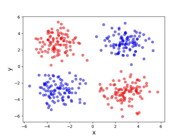
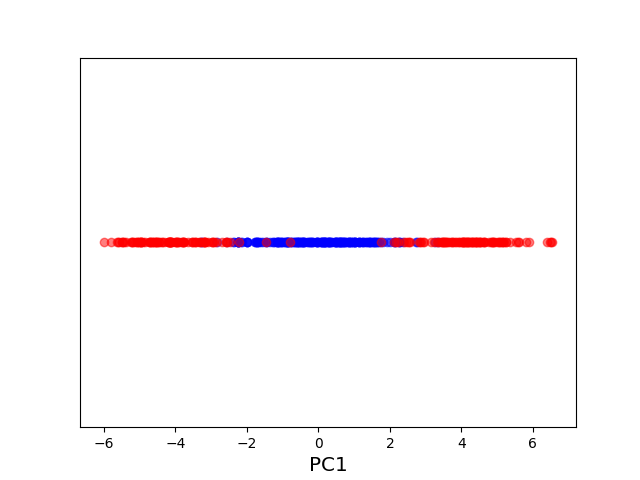
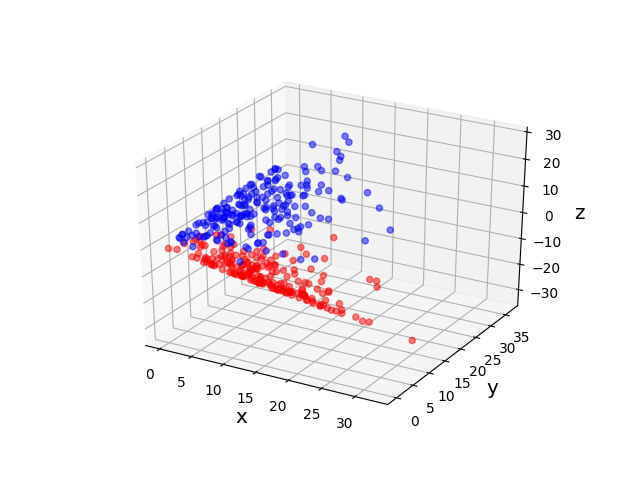
The original data set in the above example is not linearly separable, and a naive application of PCA effectively “smashes” the data and destroys its structure. After applying a non-linear “feature map” \(\phi\) to map our data from the original space \(\mathcal X = \mathbb R^2\) into the higher dimensional space \(\mathcal H = \mathbb R^3\), the resulting higher dimensional representation of the data becomes linearly separable. We can then apply PCA to obtain an embedding into the real line that respects the non-linear structure of the original data. The moral of this example is that, in order to get a good lower-dimensional representation, we had to take the intermediate step of mapping the data into a higher-dimensional feature space.

The issue with the above technique is that the dimension of the feature space \(\mathcal H\) may be so high that it becomes impractical or even impossible to explicitly evaluate the feature map \(\phi\). Let’s suppose we map our data \(\mathcal X\) into some feature space \(\mathcal H\) of (possibly infinite) dimension \(d\) via the feature map \(\phi: \mathcal X \rightarrow \mathcal H\). The data set \(\mathcal X\) could then be represented as a “matrix” \(\Phi \in \mathbb R^{m \times d}\), whose i^th row is \(\phi(\mathbf x_i)\) (I’ve used scare quotes since \(d\) is possibly infinite). As in the case of dual PCA, we cannot form the \(d \times d\) covariance matrix. Instead, we consider the Gram matrix \(\Phi \Phi^T \in \mathbb R^{m \times m}\), whose (i,j)^th entry is just the inner product \(\langle \phi(\mathbf x_i), \phi(\mathbf x_j)\rangle_{\mathcal H}\), and then proceed in the same manner as before. In other words, we are unable to explicitly calculate the principal components of the data, which belong to the potentially inaccessible feature space \(\mathcal H\). Nevertheless, we can still project the data onto the top \(k\) principal components \(\mathbf v_1, \mathbf v_2, \ldots, \mathbf v_k\) and find the coordinates of this projection in the basis \(\beta = \{\mathbf v_1, \mathbf v_2, \ldots, \mathbf v_k\}\). This clever maneuver is known as the “kernel trick,” and kernel PCA is simply a generalization of dual PCA that allows the use of non-linear kernels.

Now that I’ve described the intuition behind kernel PCA, I’m going to introduce some rigor to the discussion (my presentation will mirror [4]). Typically, the feature space \(\mathcal H\) is an \(\mathbb R\)-Hilbert space, a real inner product space that is also a complete metric space with respect to the metric induced by the inner product. Loosely speaking, Hilbert spaces are spaces which have a well-defined notion of the angle between two elements, and in which a few basic intuitions about distance hold true. A kernel on the set \(\mathcal X\) is a function \(k: \mathcal X \times \mathcal X \rightarrow \mathbb R\) satisfying

• symmetry: \[k(\mathbf x, \mathbf y) = k(\mathbf y, \mathbf x), \quad \forall \mathbf x, \mathbf y \in \mathcal X\]
• the property \[ \sum_{i=1}^\ell \sum_{j=1}^\ell \alpha_i \alpha_j k(\mathbf x_i, \mathbf x_j) \geq 0, \] \(\forall \ell > 0, (\alpha_1, \alpha_2, \ldots, \alpha_\ell)\in \mathbb R^\ell, (\mathbf x_1, \mathbf x_2, \ldots, \mathbf x_\ell) \in \mathcal X^\ell\).

An equivalent characterization of a kernel is any symmetric function \(k: \mathcal X \times \mathcal X \rightarrow \mathbb R\) such that, for any positive natural number \(\ell\) and any collection of \(\ell\) data points \(\mathbf x_1, \mathbf x_2, \ldots, \mathbf x_\ell\) from \(\mathcal X\), the Gram matrix \(K \in \mathbb R^{\ell \times \ell}\) defined by \[ K_{ij} = k(\mathbf x_i, \mathbf x_j), \quad 1 \leq i, j \leq \ell \] is a positive semi-definite matrix.

The magic of kernels is that they allow us to compute inner products in high-dimensional feature spaces. This fact is made clear by the following result from functional analysis known as Mercer’s Theorem (Note: I have not stated the theorem in full generality, but have instead provided a simplified version to get the idea across).

While the details of the theorem are somewhat involved, its significance in the current context is straightforward. Let’s suppose \(\mathcal X\) and \(k\) satisfy the conditions of the theorem, namely,

• \(\mathcal X\) is a compact subset of \(\mathbb R^n\),
• \(k\) is continuous,
• \(T_k\) is positive semi-definite (this last condition is known as Mercer’s condition).

Then we can define \(\mathcal H := \ell^2\), the \(\mathbb R\)-Hilbert space of square summable sequences in \(\mathbb R\), and \(\mathcal \phi: \mathcal X \rightarrow \mathcal H\) by the sequence \[ \phi(\mathbf x) := (\sqrt{\lambda_1} \psi_1(\mathbf x), \sqrt{\lambda_2} \psi_2(\mathbf x), \ldots). \] So by the theorem, \[ k(\mathbf x, \mathbf y) = \langle \phi(\mathbf x), \phi(\mathbf y) \rangle_{\mathcal H}, \quad \forall \mathbf x, \mathbf y \in \mathcal X. \] In other words, Mercer’s Theorem ensures that there exists an \(\mathbb R\)-Hilbert space (namely, \(\mathcal H = \ell^2\)) and a feature map \(\phi: \mathcal X \rightarrow \mathcal H\) such that the kernel \(k\) computes inner products between images of the feature map \(\phi\) in \(\mathcal H\). Moreover, the theorem provides a practical criterion to justify the use of any particular kernel. As long as a kernel satisfies the conditions of the theorem (in particular, Mercer’s condition), then we need not explicitly describe the corresponding feature map \(\phi\) (which may be an arduous task), but can rest assured that such a feature map does indeed exist. Finally, Mercer’s Theorem provides an appealing interpretation for the quantity computed by the kernel \(k\). According to the theorem, kernels compute inner products in \(\mathcal H\), which are intimately related via the Law of Cosines to the notion of angles between elements in \(\mathcal H\). Angles, in turn, can be thought of as a measure of “closeness” or “similarity.” Thus, we can aptly describe kernels as computing the similarity between high-dimensional representations of elements in our data set.

Of course, the theory developed above is useful only insofar as there exist kernels corresponding to useful feature spaces and feature maps. Here are three commonly used kernels and one lesser-known kernel:

1. We're already familiar with the simplest kernel of all, the linear kernel, and have seen its utility in the context of dual PCA. In the case of the linear kernel, the original feature space and \(\mathbb R\)-Hilbert space are identical (i.e., \(\mathcal X = \mathcal H = \mathbb R^n\)), the feature map \(\phi\) is the identity function on \(\mathbb R^n\), and the inner product \(\langle \cdot, \cdot \rangle_{\mathcal H}\) is just the standard dot product on \(\mathbb R^n\).
2. The toy example in Figure 2 uses a feature map corresponding to the so-called polynomial kernel \[ k_{\mathrm{poly}}(\mathbf x, \mathbf y) = (\langle\mathbf x, \mathbf y\rangle + c)^d \] for \(c = 0\) and \(d = 2\). In this case, the original feature space is \(\mathcal X = \mathbb R^2\), the \(\mathbb R\)-Hilbert space is \(\mathcal H = \mathbb R^3\), and the feature map \(\phi: \mathcal X \rightarrow \mathcal H\) is given by \[ \phi(x, y) = (x^2, y^2, \sqrt 2 xy). \]
3. The most commonly used non-linear kernel is the so-called radial basis function (RBF) kernel \[ k_{\mathrm{rbf}}(\mathbf x, \mathbf y) = \exp\left(-\gamma\lVert \mathbf x - \mathbf y \rVert_2^2\right), \] where \(\gamma > 0\) is a parameter. Intuitively, the RBF kernel computes the similarity between two data points. If \(\mathbf x\) and \(\mathbf y\) are close together, then the distance between these points will be small and hence the value of \(k_{\mathrm{rbf}}(\mathbf x, \mathbf y)\) will be close to 1. On the other hand, if \(\mathbf x\) and \(\mathbf y\) are far apart, then the distance between them will be large and the value of \(k_{\mathrm{rbf}}(\mathbf x, \mathbf y)\) will be close to zero. The parameter \(\gamma\) controls the scale of distance that is considered small vs. large.
   
   As in the case of the quadratic polynomial kernel, you can explicitly describe the feature map corresponding to the RBF kernel, as described in this Stack Exchange post .
4. A less common kernel is the so-called Laplacian kernel \[ k_{\mathrm{L}}(\mathbf x, \mathbf y) = \exp(-\gamma \lVert \mathbf x - \mathbf y \rVert_1), \] which has a similar interpretation to the RBF kernel.

In the context of genomic data, I’ll use the RBF kernel in my computation of kernel PCA (since Manhattan distance is equal to squared Euclidean distance in the current case, the RBF kernel is the same as the Laplacian kernel). We can estimate the variance of the data by the median of the entries in the squared pairwise distance matrix \(D_{sq}\) (call this median \(\sigma^2\)) and then set \(\gamma := 1 / (2 \sigma^2)\). Once the Gram matrix for the RBF kernel has been computed, the computation of kernel PCA proceeds in a similar manner to dual PCA. In particular, the feature map \(\phi\) corresponding to the RBF kernel is not guaranteed to result in mean-centered data. It’s thus necessary to center the data in the new feature space \(\mathcal H\) by computing the centered kernel \[ K_c = \left(I_m - \dfrac{\mathbf{1}_m \mathbf{1}_m^T}{m}\right) K \left(I_m - \dfrac{\mathbf{1}_m \mathbf{1}_m^T}{m}\right). \]

import numpy as np
from numpy.linalg import svd

def rbf_kernel_pca(D_sq, gamma, num_comp):
    m = D_sq.shape[0]
    K = np.exp(-gamma * D_sq)
    K_c = (np.eye(m) - 1 / m) @ K @ (np.eye(m) - 1 / m)
    U, Sigma_sq, _ = svd(K_c)
    Sigma = np.sqrt(Sigma_sq[:num_comp])
    return U[:,:num_comp] * Sigma

The resulting non-linear embedding of the data into two and three dimensions can be viewed in the next section.

Visualization

Due to the large number of populations included in the 1000 Genomes Project, it’s difficult to get a feel for the data using standard Python plotting libraries such as matplotlib. I thus created a Dash app to display the interactive Plotly graph displayed below. Dropdown menus allow the user to select the type of PCA (dual or kernel), whether to include or exclude the X and Y chromosomes, and which set of classes to group the data by (population, super population, or gender). You can click and drag to rotate the plot in three dimensions and zoom in and out using the scroll feature on your mouse or trackpad. You can also click on each class in the legend on the right to display or hide that class in the graph. Double-clicking will display only points from a particular class and hide points from all other classes. To get more information about a particular data point, simply hover the cursor above the point to view its coordinates and class.

Note: If your browser has difficulty loading the app, or if you’re using a smartphone and the plot is too small, you can view the 3D plot here and the 2D plot here.

The above plot provides several fascinating insights into the data. First, I was surprised to discover that the plots for dual and kernel PCA look more or less the same. This is not in general the case, and I suspect that the observed similarity is a result of the high dimension of the original feature space coupled with the sparse nature of the data. Second, when both sex chromosomes are included, the first principal component of the data is clearly interpretable as a gender axis. Male and female genomes appear to belong to distinct planes clearly separated along the first principal component, with a “V”-like structure mirrored in both planes.

When the sex chromosomes are excluded, each of the five super populations appears to have its own locus in the graph, although some super populations are more disperse than others (in particular, the class of Admixed Americans is quite spread out, an observation that accords with the diversity of heritages found in this super population). Moreover, the African, European, and Admixed American super populations (which historically have had close interactions through colonization and the slave trade) form a plane, with populations of mixed heritage appearing in intermediate locations. For example, the African-American and Afro-Caribbean populations lie mostly on the axis between the native European and native African populations, while Colombians occupy an intermediate position between all three super population loci. In contrast, the East and South Asian super populations do not have the same history of outside interaction and appear as relatively isolated clusters. Lastly, the data appears to resolve even geographically proximate populations into distinct clusters (for example, West African populations can be separated into nearby yet discernible clusters).

A PCA using only the top two principal components is displayed below.

Unlike the aforementioned study of European genomes, the two-dimensional embedding of the 1000 Genomes data set does not reproduce an easily recognizable geographical map. It’s initially tempting to interpret the first principal component (the horizontal axis in the above graph) as representing latitude; after all, the native African populations appear on the far right-hand side of the graph, and all of these populations belong either to the southern hemisphere or very near the equator. Yet this interpretation does not withstand further analysis, since other southern latitude populations such as the Lima Peruvians are actually situated to the far left of the graph.

I can think of several reasons that might account for why PCA fails to produce a recognizable world map in the current case, the first of which is a simple matter of geometry. The European subcontinent constitutes a sufficiently small portion of the Earth’s surface that it can be treated for all intents and purposes as a plane. In contrast, the entire surface of the Earth is not homeomorphic to the plane, but instead “wraps around” as longitude increases. There is thus no isometry from the sphere to the plane, so we shouldn’t expect PCA to produce an interpretable embedding into two dimensions. Secondly, the populations in the European study are geographically proximate and have a long history of close interaction. With the exception of the British Isles and a few other notable islands, Europe is a single contiguous landmass with freedom of movement unhindered within the Schengen Area. Under these conditions, the extent to which two populations interact and produce offspring of mixed heritage is largely a function of geographic distance. In contrast, the populations studied in the 1000 Genomes Project are typically isolated from one another, often separated by oceans or vast distances, and in many cases, have little history of interaction with other populations in the study. Under these circumstances, I would not expect the correlation between genetic and geographic distance to be as strong as in the European study.

Remark

In the current application, the number of samples \(m = 2504\) was small enough so that the Gram matrix easily fit in memory and its eigendecomposition could be quickly computed. If we had more samples, we could have resorted to an approximative technique such as the Nyström extension to estimate the top eigenvectors of the Gram matrix without explicitly computing the matrix itself.

References

[1] Novembre, John, et al. “Genes Mirror Geography Within Europe.” Nature 456.7218 (2008): 98.

[2] Lewis, B. W. “1000_genomes_examples.” Github, 20 July 2017, https://github.com/bwlewis/1000_genomes_examples.

[3] amoeba. “What’s the difference between principal component analysis and multidimensional scaling?” Cross Validated, https://stats.stackexchange.com/q/132731.

[4] Rudin, Cynthia. “Kernels.” Course Notes for MIT 15.097, https://ocw.mit.edu/courses/sloan-school-of-management/15-097-prediction-machine-learning-and-statistics-spring-2012/lecture-notes/MIT15_097S12_lec13.pdf.